As we enter the new year, consumers, workplaces, and schools continue to rely on video conference applications. We previously studied Bandwidth Usage of Popular Video Conferencing Applications in November 2020 and February 2021.  In May 2021, we studied Hourly Data Consumption of Popular Video Conferencing Applications. Today, we share a study of bandwidth usage on a 50Mbps/10Mbps Service Tier by popular video conferencing applications and how they perform with the addition of background traffic in the upstream.

This blog is a snapshot of the conference applications' bandwidth usage in December 2021.

The current testing used a 50 Mbps downstream and 10 Mbps upstream service tier, which doubles the upstream speed from the previous work with a 50/5 Mbps tier. With the faster upstream tier, this effort looks at both

• Bandwidth consumed for 10 concurrent conference sessions, and
• The behavior of 10 concurrent conference sessions in the presence of additional upstream traffic, specifically an upstream 5 Mbps UDP (user datagram protocol) flow.

Apple FaceTime, Google Meet, and Zoom were examined. When possible, we tested the available desktop version of each video conference application.  To avoid any appearance of endorsement of a particular conferencing application, we do not label the figures below with the specific application under test. As described below, in the presence of the 5 Mbps UDP flow in the upstream the three applications behave similarly and without any negative impact to the video-conferencing application.

In addition to the video conferencing streams, we add a 5 Mbps UDP stream of upstream traffic in the background to illustrate the capability of a 10 Mbps upstream tier. Besides video conferencing applications, other popular activities that drive upstream usage are online gaming, Wi-Fi connected cameras, and file uploads. The additional 5 Mbps stream is meant to capture a wide range of common use cases. For example, concurrent use of one to two online gaming sessions (100 to 500 Kbps each), three to four Wi-Fi connected cameras (500 Kbps to 1 Mbps each), and a file upload of 2 Mbps (900 megabytes over an hour) would all fit within this 5 Mbps upstream budget. As we show below, even with this 5 Mbps traffic and 10 concurrent sessions of the video conferencing applications, there is still upstream bandwidth available for additional activity by a subscriber with a 50 Mbps/10 Mbps service tier.

The lab setup was modified from our previous testing. The ten laptops used during this testing were different than the previous blogs; this group of laptops consisted of five MacOS and five Windows 10 operating systems. The laptops were standard consumer grade laptops without any upgrades such as those commonly used by gamers.

What did not change is the same DOCSIS 3.0 Technicolor TC8305c gateway and same CommScope E6000 cable modem termination system (CMTS) from the previous testing were used during this testing. Additionally, like the previous testing, all the laptops used wired Ethernet connections through a switch to the gateway to ensure no variables outside the control of the broadband provider would impact the speeds delivered (e.g., all the variables associated with Wi-Fi performance).  Throughout testing, we ensured there was active movement in view of each laptop’s camera to simulate real-world use cases more fully.

As in the previous blogs, this research does not consider the potential external factors that can affect Internet performance in a real home -- from the use of Wi-Fi, to building materials, to Wi-Fi interference, to the age and condition of the user’s connected devices -- but it does provide a helpful illustration of the baseline capabilities of a 50/10 Mbps broadband service.

As before, the broadband speeds were over-provisioned. For this testing, the 50/10 broadband service was over-provisioned by 25%, a typical cable operator configuration for this service tier.

To establish a baseline, we began by repeating the data collections from the three previous efforts and were able to confirm the results.  In the seven months since our last testing, many of the application developers issued updates to the applications, thus we compared the current observations with past observations looking for consistency instead of identical results.

Conferencing Application A

Figure 1 shows total access network usage for the 10 concurrent sessions over 350 seconds while using App A. The blue line is the total downstream usage, and the orange line is total upstream usage. Note that even with a 10 Mbps upstream tier, the total upstream usage stays around 2.5 Mbps. The downstream usage stays, on average, around 18 Mbps, which leaves roughly 32 Mbps of downstream headroom for other services, such as streaming video, that can use the broadband connection at the same time.

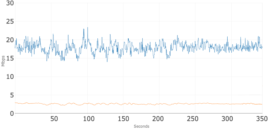
Figure 2 shows total access network usage for the 10 concurrent sessions and the addition of 5 Mbps of upstream traffic over 350 seconds while using App A. The blue line is the total downstream usage, and the orange line is total upstream usage. Note that before the upstream 5 Mbps was applied the total upstream usage was around 2.5 Mbps. At about 60 seconds, the additional 5 Mbps UDP stream was added to the upstream which causes the total to increase to about 7.5 Mbps.  As shown in Figure 3, the addition of 5 Mbps of traffic causes no noticeable impact on the upstream conference flows. At about 320 seconds that 5 Mbps stream is removed, and the upstream usage goes immediately back to where it was before that stream was applied. During the entire test the downstream usage stays, on average, around 18 Mbps even when the additional upstream bandwidth is consumed.

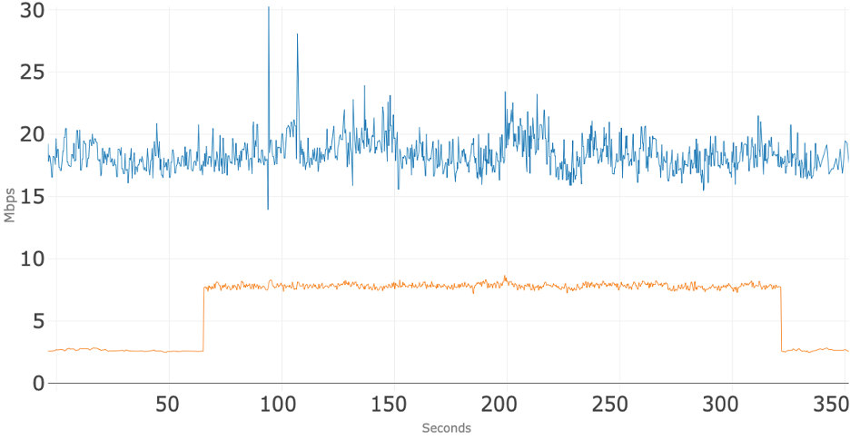
Figure 3 shows just upstream usage where the upstream traffic for the 10 concurrent sessions of App A is shown with dark orange, and the additional 5 Mbps of upstream traffic is shown in light orange. This view emphasizes that the additional 5 Mbps of upstream traffic does not appear to have an impact on the upstream bandwidth usage of the 10 concurrent video sessions of App A.

Conferencing Application B

Figure 4 shows total access network usage for the 10 concurrent sessions over 350 seconds while using App B. The blue line is the total downstream usage, and the orange line is total upstream usage. Note that even with a 10 Mbps upstream tier, the total upstream usage stays under 2.5 Mbps. The downstream usage stays, on average, around 13 Mbps, which leaves roughly 37 Mbps of downstream headroom for other services.

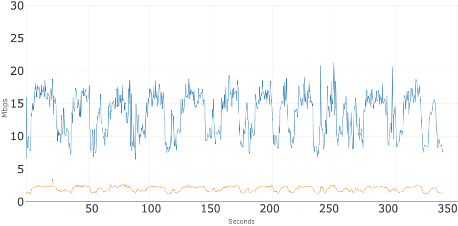
Figure 5 shows total access network usage for the 10 concurrent sessions and the addition of 5 Mbps of upstream traffic over 350 seconds while using App B. The blue line is the total downstream usage, and the orange line is total upstream usage. Note that before the upstream 5 Mbps was applied the total upstream usage was around 2.5 Mbps. At about 60 seconds, an additional 5 Mbps stream was added to the upstream which causes the total to increase to about 7 Mbps.  As shown in Figure 6, the addition of the 5 Mbps of traffic causes no noticeable impact on the upstream conference flows. At about 270 seconds that 5 Mbps stream is removed, and the upstream usage goes immediately to where it was before that stream was applied. During the test the downstream usage stays, on average, around 13 Mbps even when the additional upstream bandwidth is consumed.

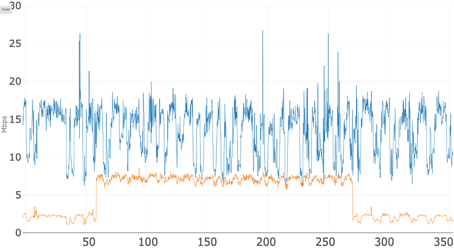
Figure 6 shows just upstream usage where the upstream traffic for the 10 concurrent sessions of App B is shown with dark orange, and the additional 5 Mbps of upstream traffic is shown in light orange. This view demonstrates that the additional 5 Mbps of upstream traffic does not appear to have an impact on data usage of the 10 concurrent video sessions of App B.

Conferencing Application C

Figure 7 shows total access network usage for the 10 concurrent sessions over 350 seconds while using App C. The blue line is the total downstream usage, and the orange line is total upstream usage. Note that even with a 10 Mbps upstream tier, the total upstream usage stays around 4 Mbps. The downstream usage stays, on average, around 10 Mbps, which leaves roughly 40 Mbps of downstream headroom for other services.

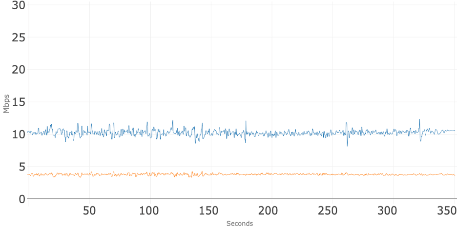
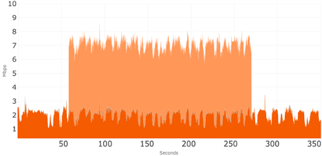
Figure 8 shows total access network usage for the 10 concurrent sessions and the addition of 5 Mbps of upstream traffic over 350 seconds while using App C. The blue line is the total downstream usage, and the orange line is total upstream usage. Note that before the upstream 5 Mbps was applied the total upstream usage was around 4 Mbps. At about 70 seconds, an additional 5 Mbps stream was added to the upstream which causes the total to increase to about 9 Mbps.  As shown in Figure 9, the addition of the 5 Mbps of traffic causes no noticeable impact on the upstream conference flows. At about 260 seconds that 5 Mbps stream is removed, and the upstream usage goes immediately back to where it was before that stream was applied. During the entire test, the downstream usage stays, on average, around 10 Mbps even when the additional upstream bandwidth is consumed.

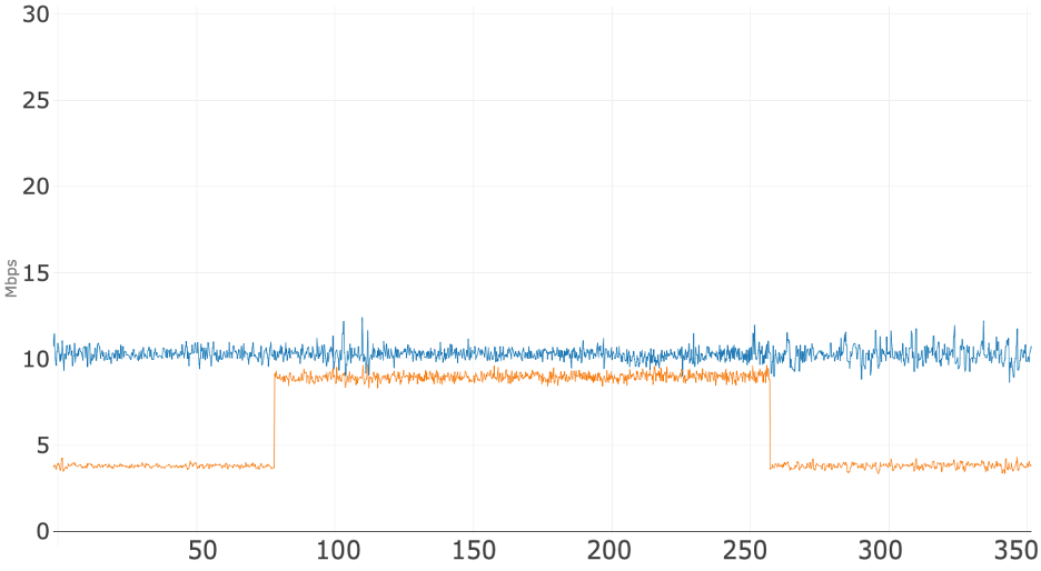
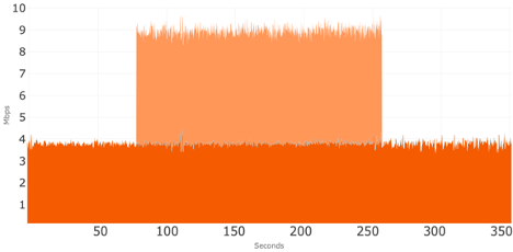
Figure 9 shows just upstream usage where the upstream traffic for the 10 concurrent sessions of App C is shown with dark orange, and the additional 5 Mbps of upstream traffic is shown in light orange. This view demonstrates that the additional 5 Mbps of upstream traffic does not appear to have an impact on the data usage of the 10 concurrent video sessions of App C.

Summary

This investigation looked at three popular video conferencing applications over an upstream tier of 10 Mbps and a downstream tier of 50 Mbps.

The three applications exhibited similar behavior of using under 4 Mbps of upstream during 10 concurrent conference sessions. When an additional 5 Mbps of upstream traffic was added, these three conference apps took it in stride; there were no noticeable changes to either the upstream or downstream consumption of the 10 concurrent conference sessions and no negative impact to the quality of the video conferencing sessions.

The successful testing of 10 concurrent video sessions plus 5 Mbps of additional background traffic illustrates the capability of a 50/10 service tier to support the broadband needs of telework, remote education, telehealth, and other use cases that rely heavily on video conferencing applications. The testing also illustrates that a 50/10 service tier can readily support a household with multiple users engaging on video conference platforms as well as support other simultaneous uses.

As consumers’ bandwidth needs continue to grow, cable operators are always thinking of ways to expand their network capacity to accommodate future increases in data traffic—especially upstream traffic. Band splits play an important role in that effort, taking advantage of the incredible resiliency of cable’s hybrid fiber-coaxial (HFC) network.

What Is a Band Split and How Does It Work?

To describe what band splits are, we need to first define bandwidth. The best way to think of bandwidth is as a stretchable pipe that allows radio frequency (RF) signals carrying data to travel through it. So, when we talk about expanding the bandwidth of a network, we’re looking for ways to stretch that pipe to higher frequencies to accommodate more data traffic. The term “bandwidth” is somewhat synonymous with “capacity,” and on cable networks bandwidth is measured in megahertz (MHz) and gigahertz (GHz)—1 GHz is 1,000 times greater than 1 MHz.

The following figure shows several options available for band splits on the cable broadband network, allowing various mixes of upstream and downstream bandwidth depending on the needs of consumers. Frequency Division Duplex (FDD) designates separate bands for upstream and downstream traffic.

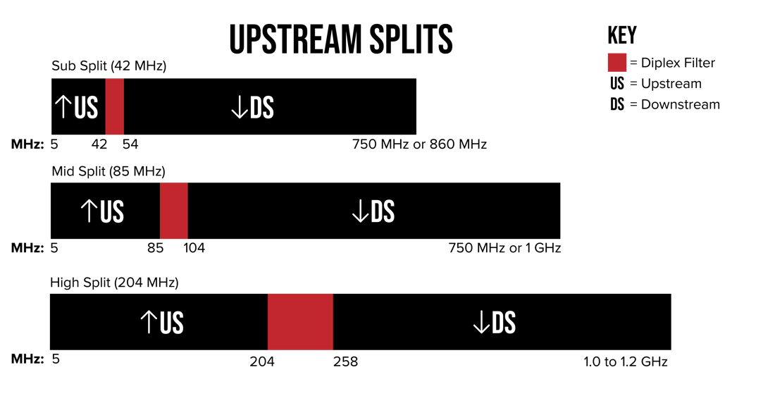
The bandwidth “pipe” (split into two parts) has data traffic traveling in opposite directions: downstream from your provider’s hub to your modem and upstream from your modem back to the hub. This back-and-forth flow allows you to use interactive services like video chat, teleconferencing, telehealth and more.

Band splits determine how much bandwidth is dedicated to downstream and upstream channels. Downstream traffic is usually transmitted on a high-band frequency range, whereas the lower band is dedicated to upstream traffic. Two-way amplifiers are used to amplify signals in both directions. These amplifiers have something called diplex filters to separate downstream and upstream frequencies to prevent interference.

Usually, consumers use a much larger chunk of the bandwidth pipe for downstream traffic, but that’s starting to change. As people switch to working and studying from home, they’re using more interactive services like video chats, which require more upstream data. To accommodate this trend and future demand, network operators need to consider when to add more upstream bandwidth. For this reason, they may need to rethink the way their networks are split.

What Kind of Band Splits Are There?

Not all band splits are created equal: In North America, there are sub-splits, mid-splits and high-splits, and Europe has its own band split. This situation has to do with how the operator divides the available bandwidth pipe between downstream and upstream traffic.

Although sub-splits are still prevalent in North America today, mid-split and high-split bands require an upgrade. In a sub-split, a spectrum range of 5 MHz to 42 MHz is used for upstream traffic and 54 MHz to 1.2 GHz or 1.8 GHz is for downstream traffic. In a mid-split scenario, 5 MHz to 85 MHz is dedicated for upstream and above 108 MHz for downstream. And high-split extends the upstream range to 204 MHz while reserving 258 MHz and higher frequencies for downstream.

The European split uses an upstream spectrum range of 5 MHz to 65 MHz, and the downstream spectrum range is above 88 MHz. There’s also an ultra-high-split where the upstream goes to a 684 MHz upper-frequency limit that includes even more choices of band-splits, which some operators may consider in the future. However, for most networks in North America, Europe and Latin America, future bandwidth allocations will consist of mid-split and high-split bands, and even some ultra-high-splits.

How Has This Technology Evolved?

If we go back to the early pre-internet days, information on cable networks traveled one way, delivering analog TV signals to millions of homes over coaxial cable, with no data traveling back from the consumer to the hub. Eventually, as consumer needs evolved, so did the industry, and networks began to send signals both ways, to and from the consumer, opening doors to cable broadband Internet, video chatting and much, much more.

As we move toward the next phase of HFC evolution, we must remember that building the super-fast and reliable networks we have today required a lot of collaboration and about $290 billion dollars in infrastructure and network investments over the past 20 years. And that’s just in the United States! For most cable operators, a re-allocation to mid-split, high-split or a mix of the two will require switching out signal amplifiers and other legacy equipment—an investment that many are already making. Although there’s no one-size-fits-all approach, the consensus is to move to at least the mid-split in the near future, further expanding the incredible capacity of the HFC network.

How Will Higher Band Splits Affect You and Your Future?

Although as a consumer you’ll never have to worry about how your cable company’s bandwidth is split between downstream and upstream, we know you pay attention to network speed. The journey from today’s 1G to tomorrow’s 10G offerings will involve expanding the bandwidth pipe to allow for more capacity. More bandwidth will give us more flexibility to accommodate near-future technologies, including bandwidth-hungry virtual reality (VR) applications and more.

That’s where band splitting really makes a difference. Dedicating higher band splits to upstream traffic will future-proof our networks for years to come, allowing us to reach our goals and build the next-generation of technologies to help us live, work, learn and play in the coming decades.

Building on our prior work, this investigation explores the hourly data consumption of popular video conferencing applications: Google Meet, GoToMeeting, Microsoft Teams and Zoom. As video conference applications have become an integral part of our daily lives, we wanted to not only better understand the bandwidth usage as previously explored, but also the total data consumption of these applications. This investigation provides a first step in better understanding that latter dimension. To avoid any appearance of endorsement of a particular conferencing application, we have not labeled the figures below with the specific apps under test. In short, we observed that a single user on a video conferencing application consumed roughly one gigabyte per hour, which compares to about three gigabytes per hour when streaming an HD movie or other video. However, we did observe substantial variance in video conferencing app hourly data consumption based on the specific app and end-user device.

Key Components of the Testing Environment

Much like our prior work on bandwidth usage, the test setup used typical settings and looked at both upstream and downstream data consumption from laptops connected to a cable broadband internet service. We used the same network equipment from November and our more recent blog post in February. This includes the same cable equipment as the previous blogs — the same DOCSIS 3.0 Technicolor TC8305c gateway, supporting eight downstream channels and four upstream channels, and the same CommScope E6000 cable modem termination system (CMTS). The cable network was configured to provide 50 Mbps downstream and five Mbps upstream broadband service, overprovisioned by 25 percent.

The data gathering scenario:

1. 10 people, each on their individual laptops, participated in the conference under test
2. One person on the broadband connection under test, using either a lower-cost or a higher-cost laptop. The other nine participants were not using the broadband connection under test.
3. For the laptop under test, the participant used the video conferencing application for the laptop’s operating system, rather than using the video conferencing application through the web browser.
4. Total data consumption was recorded for the laptop using the broadband connection under test.

For all 10 participants, cameras and microphones were on. Conference applications were set to "gallery mode" with thumbnails of each person filling the screen, no slides were presented and the video conference sessions just included people talking.

The laptop under test used a wired connection to the cable modem to ensure that no variables outside the control of the service provider would impact broadband performance. Most notably, by using a wired connection, we removed the variable of Wi-Fi performance from our test setup. During data collection, the conference app was the only app open on the laptop under test.

Video conferencing sessions were set up and data consumption was measured over time. We collected 10 minutes of data for each conferencing session under test to calculate the total consumption for one hour. The charts below show the data consumed for each of the 10 minutes of the conference session. During the conference there was movement and discussion to keep the video and audio streams active throughout the period of data collection.

For each test scenario, only one laptop was connected at a time to the broadband connection under test. Our goal was to measure the data consumption of one conferencing user on the broadband connection. The other conference participants were on the internet; they were not in the lab. Once again, we used TShark (a popular, widely used network protocol analyzer) to capture and measure the data.

For the laptop under test, we chose two that have quite different capabilities. The first was a low-cost laptop with an 11-inch screen, like the ones students are often provided by school districts for at-home learning. The second was a higher-cost laptop with a 15-inch screen, like what we often see in an enterprise environment. Note the two laptops not only have quite different hardware components (e.g., CPU, graphics processors, memory, cameras, screens), but also have different operating systems. Once again, to avoid any appearance of endorsement, we are not identifying the specific laptops used.

Analysis

Table 1 shows hourly bandwidth consumption (combining both upstream and downstream) for the laptop under test, normalized to Gigabytes per hour. The table provides the data consumption for the low-cost and higher-cost laptops in each scenario with the four conferencing applications.

Table 1: Video Conferencing App Hourly Bandwidth Consumption in Gigabytes for Each User (Gigabytes/hour)

The following figures show the data consumption, in Megabytes, for each minute of the 10-minute data collection for each of the permutations of our testing.

A few notes on the charts:

• There was only one client behind the cable modem.
• Each bar represents one minute of data consumption.
• Each bar shows total consumption and includes both the upstream and downstream, and both audio and video, added together.
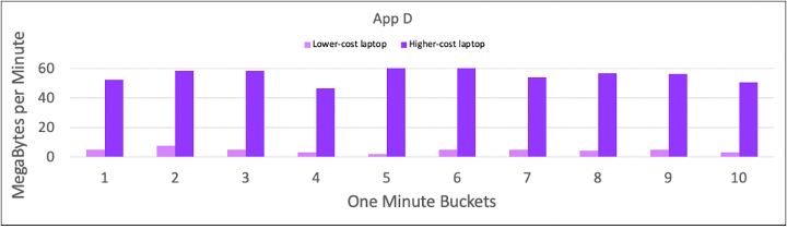
• App A is blue in each chart; App B is green; App C orange; and App D is purple.
• These charts show real-time consumption measured in Megabytes per hour to illustrate consumption over time.

Figure 1 shows the data consumed when using the lower-cost laptop in the 10-person meetings.

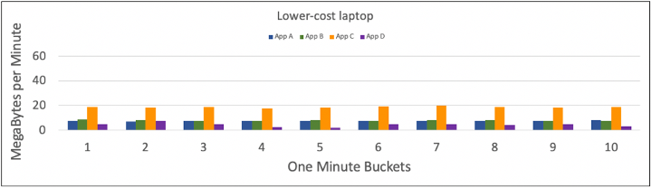
Figure 2 shows data consumed each minute for each of the four apps when using the higher-cost laptop was in the 10-person meetings.

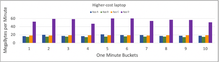
Figure 3 shows the data consumed each minute using App A and compares the two laptops used for data collection. For each minute, the bar to the left is the lower-cost laptop and the bar to the right is the higher-cost laptop.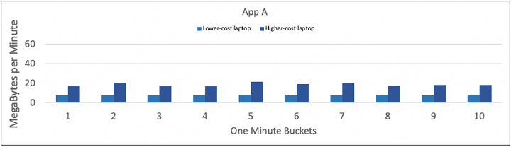

Figure 4 shows the data consumed each minute using App B and compares the two laptops. The bar to the left is the lower-cost laptop and the bar to the right is the higher-cost laptop.

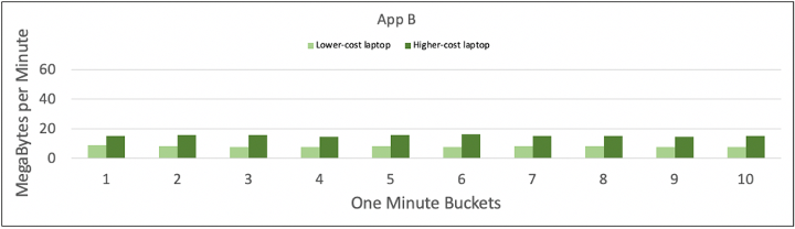
Figure 5 shows the data consumed each minute using App C and compares the two laptops. The bar to the left is the lower-cost laptop and the bar to the right is the higher-cost laptop.

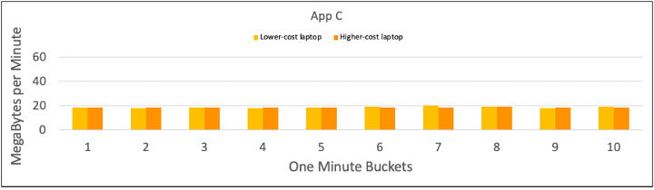
Figure 6 shows the data consumed each minute using App D and compares the two laptops. The bar to the left is the lower-cost laptop and the bar to the right is the higher-cost laptop.

Key Observations

A. Data Consumption Varies: The first takeaway is that different apps consume different amounts of bandwidth, as shown in Table 1, from 0.5 GBytes per hour up to 3.4 GBytes per hour, for video conferences using the different laptops, the same broadband connections, the same general setup (e.g., gallery view), the same people doing the same things on camera, etc.

1. 1. For a  given app on a given laptop, data consumption was consistent over the 10-minute collection time.
   2. App D using the higher-cost laptop consumed the most bandwidth.
   3. With App D on the lower-cost laptop, there was video quality degradation. We confirmed the broadband connection was operating as expected and was not the cause of the video degradation. Rather, it appeared that the combination of the hardware and operating system of the lower-cost laptop was unable to meet the resource requirements of App D.
   4. App B consistently consumed less bandwidth regardless of scenario.

B. Comparing Laptops: In Table 1, the two columns of data show the differences between the lower-cost and higher-cost laptops for the data collections. On the lower-cost laptop, Apps A, B and C consume about the same amount of data on an hourly basis.

C. Comparing Laptops: The second column of data show that all apps on the higher-cost laptop consumed more bandwidth than the lower-cost laptop. This difference implies that when using the actual conferencing app (not a web browser), processing power available in the laptop may be a determining factor in consumption.

D. Comparing Apps: App C was the most consistent in data consumption regardless of the laptop used. The other conference applications noticeably consumed more on the higher-cost laptop.

In summary, we observed a more than 7X variation in the data consumption of video conferencing with a very limited exploration of just two variables – laptop and video conferencing application. Notably, however, when data consumption was at its highest, it was of the same magnitude as the data consumption of an HD video stream.

This is an area ripe for further research and study, both to more comprehensively explore these variables (e.g., other device types, larger meetings) and to explore other variables that may meaningfully influence data consumption.

This month, we continue our CableLabs 101 series by peeling back the next layer of the hybrid fiber-coax (HFC) distributed access network with a recently released specification called Flexible MAC Architecture (FMA). This technology isn’t as well known as DOCSIS®, Remote PHY or Coherent Optics, but it’s just as essential to make 10G a reality in the near future. Let’s take a closer look.

What Is FMA?

Without getting too technical, a big part of what we do involves analyzing how things work. We like to take things apart and see how we can reorganize or alter the components to build better, more efficient products. Essentially, that’s what innovation is all about! In this case, the “product” in question is the DOCSIS technology and the cable access network that delivers Internet to your home.

Some time ago, we figured out how to split key DOCSIS functions into two major pieces: the Media Access Control (MAC) function responsible for DOCSIS processing and the physical radio frequency function (PHY) responsible for DOCSIS signal generation. This initial split became known as Remote PHY, and you can read more about it in our previous blog post here. Subsequently, we built a complementary project involving the redistribution of these functions across the network to enable efficiencies in speed, reliability, latency and security. This newer project is FMA, which defines various ways of restructuring the MAC function’s management, control and data planes to support multi-gigabit data services of the future.

In September 2020, this extraordinary effort—involving thousands of work hours across the global cable industry—culminated in the specification. It’s a library of specifications that gives our industry vendors the technical means to develop interoperable products for our cable community, and it officially welcomes FMA into the 10G technologies toolkit.

How Does FMA Work and Why Do You Need It?

The Converged Cable Access Platform (CCAP)—a nearly decade-old technology—serves as a single platform for both video and broadband services. In a traditional CCAP architecture, all the major network functions, including the MAC layer functions we mentioned earlier, are unified at the headend. However, as consumers’ bandwidth consumption has continued to skyrocket with no sign of slowing down, the cable industry asked: Is there a better way to structure CCAP to prepare our networks for the needs of tomorrow?

The answer was yes.

That’s how the concepts of Remote PHY, Remote MAC-PHY and, eventually, FMA were born. By taking apart key CCAP functions and moving them to other places throughout the network (e.g., a fiber node), we can greatly reduce space and power demands at the headend, creating efficiencies that translate into faster network speeds, lower latencies and overall a better, and reliable cable access network.

Plus, FMA offers cable operators the ultimate flexibility to implement and deploy CCAP functionality in a way that makes the most sense for them. It fully supports the DOCSIS 4.0 requirements and, along with the other tools in the 10G arsenal, can help operators build adaptive and secure networks that can easily handle future demand.

How Does This Technology Affect You and Your Future?

Complete disaggregation of CCAP sounds great, but you might be asking yourself: “What’s in it for me?” As with any 10G technology that we’ll cover in this series, it’s always about improving the end user experience. All those technical efficiencies we talked about basically boil down to more room for data to go through the network at much faster speeds. This means more multi-gigabit services, low-latency applications such as ultra-realistic video experiences and overall a better quality of experience. One day soon, as we continue to build upon cutting-edge cable technologies like FMA, this will become reality.

The September 2020 FMA release is just a part of a much bigger initiative to completely virtualize cable access networks in the near future, so definitely stay tuned! In the meantime, we’ll continue taking things apart and putting them back together in new and better ways to take your connected experiences to the next level.

In our previous CableLabs 101 post about Distributed Access Architecture (DAA), we discussed the benefits of distributing key network functions throughout the cable access network to optimize its performance. Today, we delve deeper into Remote PHY—one of the earliest DAA solutions that cable operators are deploying to increase their network’s bandwidth and more.

What Is Remote PHY?

PHY stands for “physical radio frequency (RF) layer,” which delivers voice, video and data via the DOCSIS® protocol over the hybrid fiber-coax (HFC) network. Media Access Control (MAC) is an example of another CCAP layer that we’ll cover in our next CableLabs 101 post.

Prior to the introduction of the DAA concept, all CCAP functions, including PHY and MAC, were integrated at the Internet provider’s cable modem termination system (CMTS)—typically located at the headend or hub site—which sends and receives data to and from the modem in your home. This data exchange is the basis for how DOCSIS technology on HFC networks works. However, the integrated CCAP approach does not maximize the potential of the cable access network.

Once we figured out how to split the PHY and MAC functions, we were then able to distribute PHY closer to the end user, resulting in increased network capacity and greater speeds. You can refresh your memory about the benefits of DAA and Distributed CCAP Architecture (DCA) here.

Remote PHY was the first documented DCA specification that we officially released in 2015, followed by Flexible MAC Architecture (FMA), released in September 2020. These solutions are complementary and have similar benefits, giving cable operators the flexibility to architect their networks the way they see fit to support future high-bandwidth services. The specifications provide guidance to our industry vendors who are manufacturing Remote PHY–compatible equipment. Just like the other DOCSIS and Coherent Optics technologies, Remote PHY and the other DCA approaches are part of the 10G toolset.

How Does Remote PHY Work?

The Remote PHY specification defines ways to separate the physical RF layer from the MAC layer that remains at the headend and describes the interfaces between them. Let’s take a closer look at how it’s done.

The PHY layer of the CCAP system is placed in something called a Remote PHY Device (RPD). An RPD is a piece of equipment usually produced by a third-party cable vendor that contains all the PHY-related circuitry, as well as the pseudowire logic that connects back to the CCAP Core, which supports full DOCSIS functionality. In other words, all this rerouting on the back end is completely hidden from customers like you. Your network will function the same as before, only much faster because the PHY layer is now located much closer to where you live.

Speaking of location, the beauty of the Remote PHY architecture lies in its flexibility to place RPDs anywhere, including optical nodes closer to the network “edge”—a cable insider’s way of saying “closer to customers’ homes.” A single node can serve just a few blocks or even a single building; therefore, each customer modem connected to that node gets a bigger chunk of the bandwidth pie, so to speak. And, of course, more available bandwidth means better customer experience!

How Does This Technology Affect Me and My Future?

You might think that it makes no difference to you how your Internet provider’s CCAP is designed—and you would be right. What does matter, however, is the noticeable difference in your Internet quality, including how fast your apps work, how quickly you can download your movies or how much lag (or lack thereof) you experience when you play an online game with your friends. Looking forward to the near future, you may be using applications that utilize holographic displays, artificial intelligence, virtual rooms, 360° fully immersive entertainment experiences and other innovative technologies that require multi-gigabit bandwidth to function seamlessly.

This is why CableLabs and our partners in the cable industry are continuously inventing new ways to mine more bandwidth out of the available RF spectrum. Thanks to specifications like Remote PHY, FMA and others, we have all the pieces in place to deliver 10G symmetrical speeds—and more—to support future innovations. Now it’s just a matter of putting it all together.

As working from home and remote schooling remain the norm for most of us, we wanted to build on and extend our prior investigation of the bandwidth usage of popular video conferencing applications. In this post, we examine the use of video conferencing applications over a broadband service of 50 Mbps downstream and 5 Mbps upstream (“50/5 broadband service”). The goal remains the same, looking at how many simultaneous conferencing sessions can be supported on the access network using popular video conferencing applications. As before, we examined Google Meet, GoToMeeting, and Zoom, and this time we added Microsoft Teams and an examination of a mix of these applications. To avoid any appearance of endorsement of a particular conferencing application, we haven’t labeled the figures below with the specific apps under test.

We used the same network equipment from November. This includes the same cable equipment as the previous blog -- the same DOCSIS 3.0 Technicolor TC8305c gateway, supporting 8 downstream channels and 4 upstream channels, and the same CommScope E6000 cable modem termination system (CMTS).

The same laptops were also used, though this time we increased it to 10 laptops. Various laptops were used, running Windows, MacOS and Ubuntu – nothing special, just laptops that were around the lab and available for use. All used wired Ethernet connections through a switch to the modem to ensure no variables outside the control of the broadband provider would impact the speeds delivered (e.g., placement of the Wi-Fi access point, as noted below). Conference sessions were set up and parameters varied while traffic flow rates were collected over time.  Throughout testing, we ensured there was active movement in view of each laptop’s camera to more fully simulate real-world use cases.

As in the previous blog, this research doesn’t take into account the potential external factors that can affect Internet performance in a real home -- from the use of Wi-Fi, to building materials, to Wi-Fi interference, to the age and condition of the user’s connected devices -- but it does provide a helpful illustration of the baseline capabilities of a 50/5 broadband service.

As before, the broadband speeds were over-provisioned. For this testing, the 50/5 broadband service was over provisioned by 25%, a typical configuration for this service tier.

First things first: We repeated the work from November using the 25/3 broadband service. And happily, those results were re-confirmed. We felt the baseline was important to verify the setup.

Next, we moved to the 50/5 broadband service and got to work. At a high level, we found that all four conferencing solutions could support at least 10 concurrent sessions on 10 separate laptops connected to the same cable modem with the aforementioned 50/5 broadband service and with all sessions in gallery view. The quality of all 10 sessions was good and consistent throughout, with no jitter, choppiness, artifacts or other defects noticed during the sessions. Not surprisingly, with the increase in the nominal upstream speed from 3 Mbps to 5 Mbps, we were able to increase the number of concurrent sessions from the 5 we listed in the November blog to 10 sessions with the 50/5 broadband service under test.

The data presented below represents samples that were collected every 200 milliseconds over a 5-minute interval (300 seconds) using tshark (the Wireshark network analyzer).

Conferencing Application: A

The chart below (Figure 1) shows total access network usage for the 10 concurrent sessions over 300 seconds (5 minutes) while using one of the above conferencing applications. The blue line is the total downstream usage, and the orange line is total upstream usage. Note that the total upstream usage stays around 2.5 Mbps which may be a result of running 10 concurrent sessions. Also, the downstream usage stays, on average, around 15 mbps, which leaves roughly 35 Mbps of downstream headroom for other services such as streaming video that can also use the broadband connection at the same time.

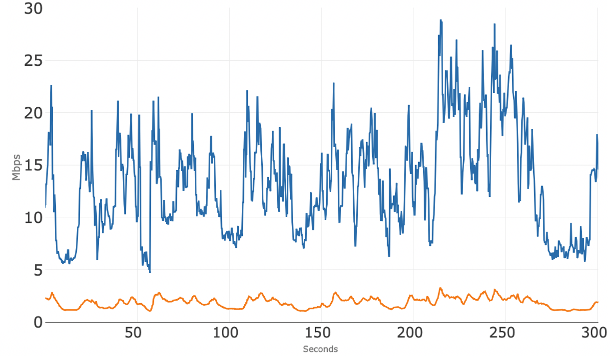
Figure 2 shows the upstream bandwidth usage of the 10 concurrent sessions and it appears that these individual sessions are competing amongst themselves for upstream bandwidth. However, all upstream sessions typically stay well below 0.5 Mbps -- these streams are all independent, with the amount of upstream bandwidth usage fluctuating over time.

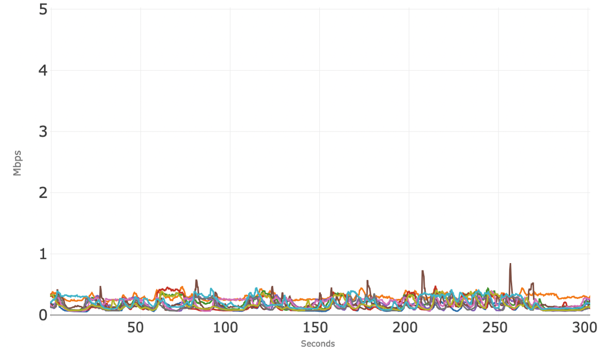
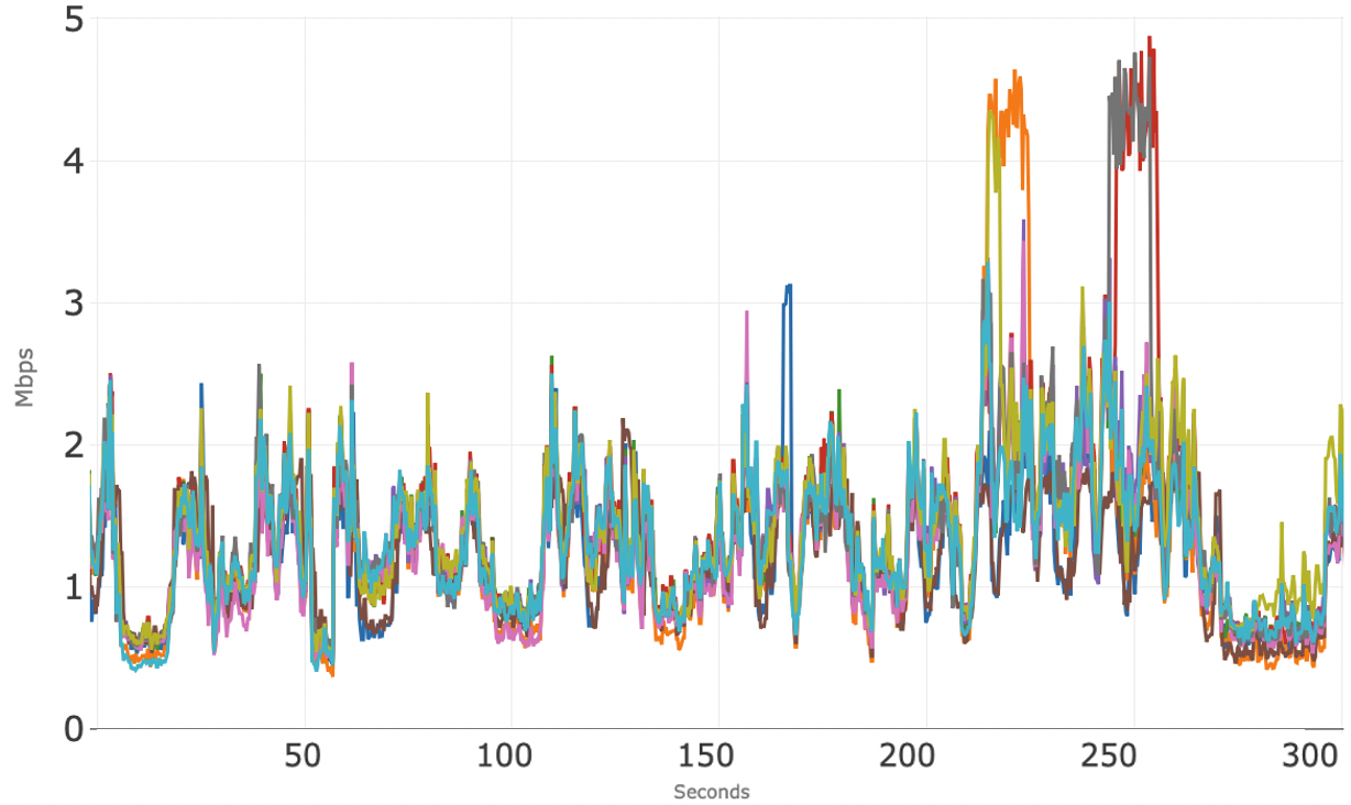
Figure 3 shows the downstream bandwidth usage for the 10 individual conference sessions. Each conference session typically uses between 1 to 2 Mbps. As previously observed with this application, there are short periods of time when some of the sessions use more downstream bandwidth than the typical 1 to 2 Mbps.

Conferencing Application: B

Figure 4 shows access network usage for 10 concurrent sessions over 300 seconds (5 minutes) for the second conferencing application tested. The blue line is the total downstream usage, and the orange line is total upstream usage. Note that the total upstream usage hovers around 3.5 Mbps.  The total downstream usage is very tight, right above 10 Mbps.

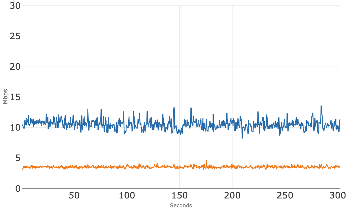
Figure 5 shows the upstream bandwidth usage of the 10 individual conference sessions where all but one session is well below 1 Mbps and that one session is right at 2 Mbps.  We don’t have an explanation for why that blue session is so much higher than the others, but it falls well within the available upstream bandwidth.

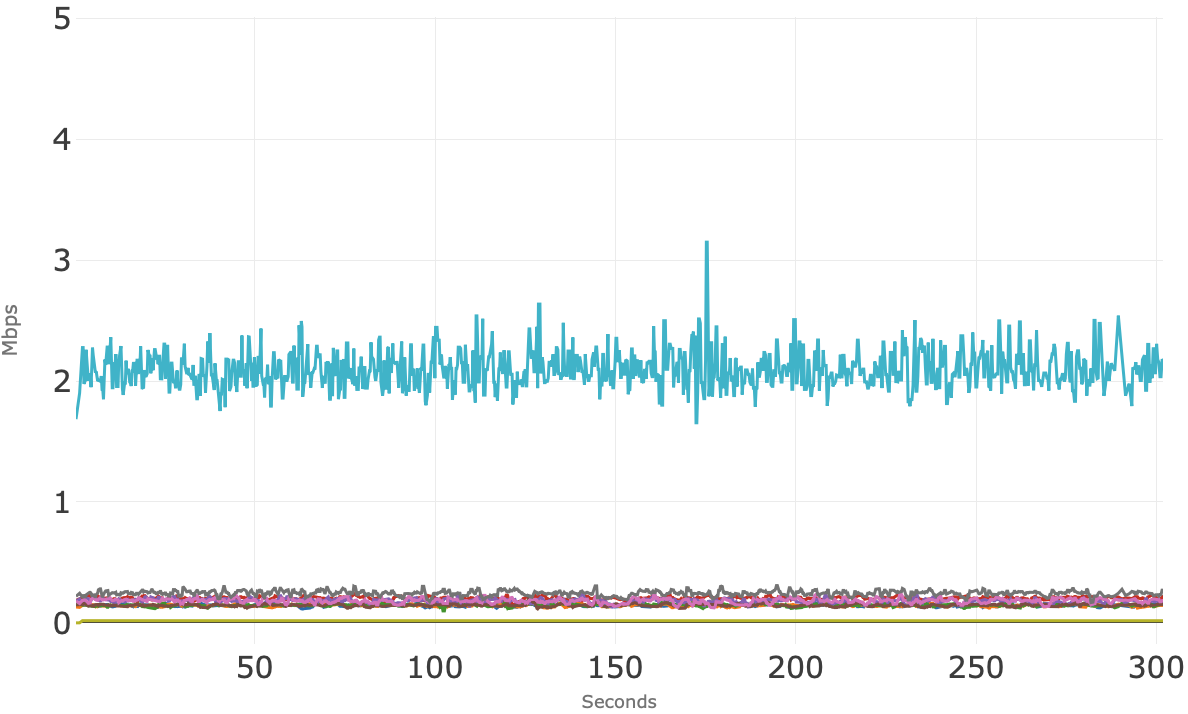
Figure 6 shows the downstream bandwidth usage for the 10 individual conference sessions clusters consistently around 1 Mbps.

Conferencing Application: C

Figure 7 shows access network usage for the 10 concurrent sessions over 300 seconds (5 minutes) for the third application tested. The blue line is the total downstream usage, and the orange line is total upstream usage. Note that the total upstream usage hovers right at 3 Mbps over the 5 minutes.

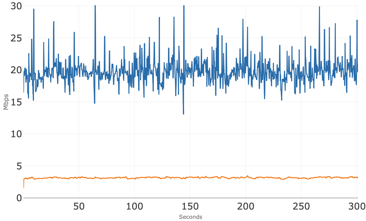
Figure 8 shows the upstream bandwidth usage of the 10 individual conference sessions where all stay well below 1 Mbps.

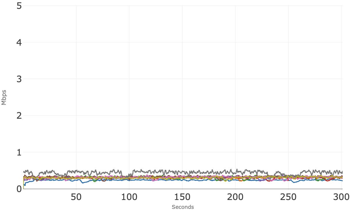
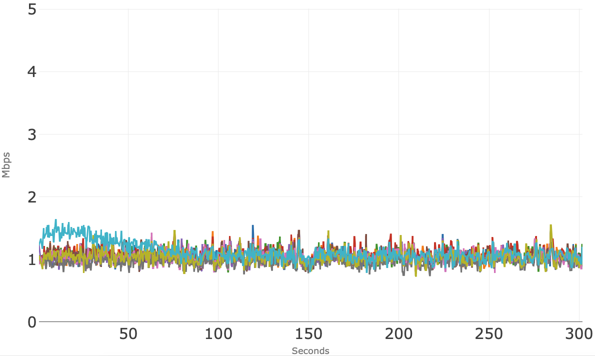
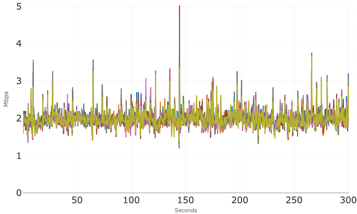
Figure 9 shows the downstream bandwidth usage for the 10 individual conference sessions. These sessions appear to track each other very closely around 2 Mbps, which matches Figure 7 showing aggregate downstream usage around 20 Mbps.

Conference Application: D

Figure 10 shows access network usage for the 10 concurrent sessions over 300 seconds (5 minutes) for the fourth application tested. The blue line is the total downstream usage, and the orange line is total upstream usage. Note that the total upstream usage hovers right at 5 Mbps over the 5 minutes, and there is no visible degradation to the conferencing sessions was observed.

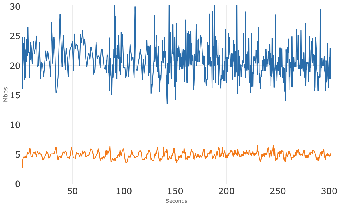
Figure 11 shows the upstream bandwidth usage of the 10 individual conference sessions, where there is some variability in bandwidth consumed per session.  One session (red) consistently uses more upstream bandwidth than the other sessions but remained well below the available upstream bandwidth.

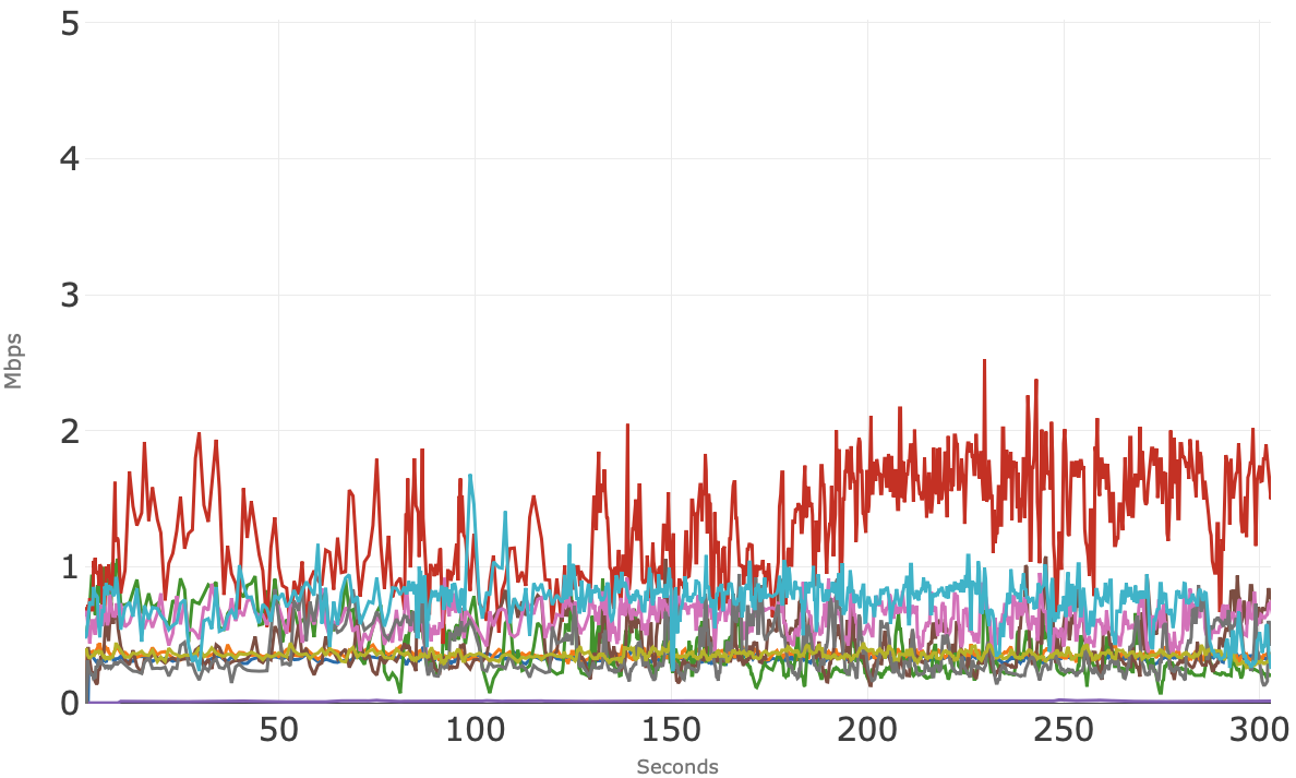
Figure 12 shows the downstream bandwidth usage for the 10 individual conference sessions. These sessions show two groups, with one group using less than 1 Mbps of bandwidth and the second group using consistently between 2 Mbps and 4 Mbps of bandwidth.

Running All Four Conference Applications Simultaneously

In this section, we examine the bandwidth usage of all four conferencing applications running simultaneously. The test consists of three concurrent sessions from two of the applications and two concurrent sessions from the other two applications (once again a total of 10 conference sessions running simultaneously). The goal is to observe how the applications may interact in the scenario where members of the same household are using different conference applications at the same time.

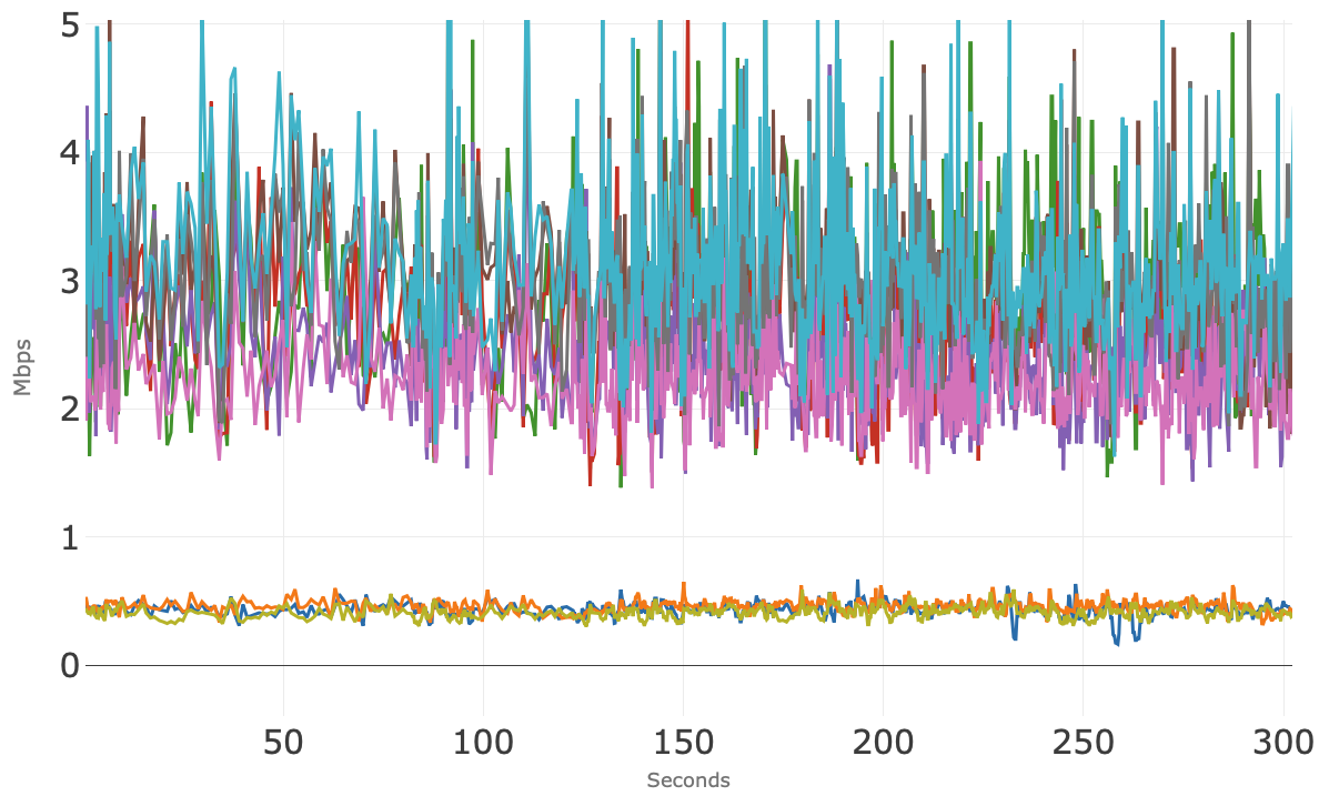
Figure 13 shows access network usage for these 10 concurrent sessions over 300 seconds (5 minutes). The blue line is the total downstream usage, and the orange line is total upstream usage. Note that the total upstream usage once again hovers around 5 Mbps without any visible degradation to the conferencing sessions, and the downstream usage is pretty tight right above 10 Mbps.

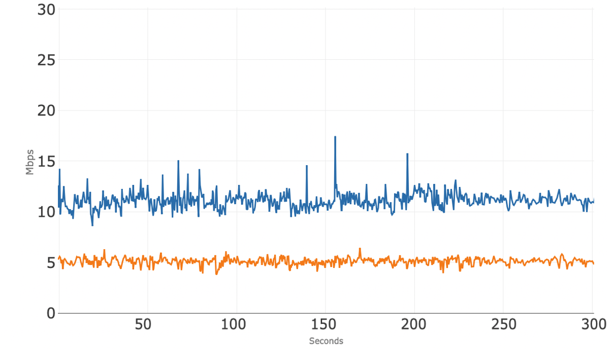
Figure 14 shows the upstream bandwidth usage of the 10 individual conference sessions where several distinct groupings of sessions are visible. There were 4 different apps running concurrently. One session (red) consumes the most upstream bandwidth at averaging around 2 Mbps, whereas the other sessions use less, and some much less.

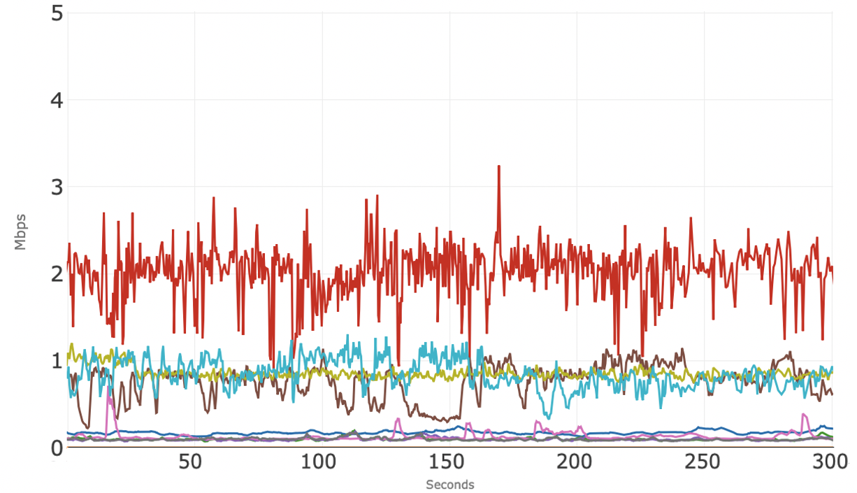
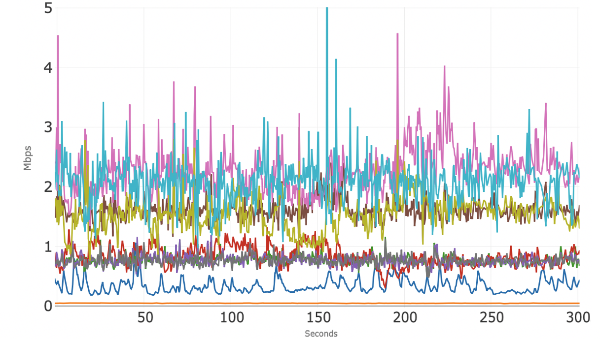
Figure 15 shows the downstream bandwidth usage for the 10 individual conference sessions across the four apps and, again, there are different clusters of sessions. Each of the four apps are following their own algorithms.

In summary, with a 50/5 broadband service, each of the video-conferencing applications supported at least 10 concurrent sessions, both when using a single conferencing application and when using a mix of these four applications. In all cases, the quality of the 10 concurrent sessions was good and consistent throughout. The 5 Mbps of nominal upstream bandwidth was sufficient to support the conferencing sessions without visible degradation, and there was more than sufficient available downstream bandwidth to run other common applications, such as video streaming and web browsing, concurrently with the 10 conferencing sessions.

This month, we’d like to share information about Distributed Access Architecture (DAA) and how cable operators are using it to build the 10G networks of the future. In our previous posts about DOCSIS® and Coherent Optics technologies, we touched on some of the components of the cable hybrid fiber-coax (HFC) network, such as the headend and fiber nodes, but of course, there’s much more to it. Today, we’ll take a closer look at the functionality of the cable access network and how it can be distributed between various components to optimize network performance.

What Is Distributed Access Architecture?

DAA isn’t a single technology but rather an umbrella term that describes the network architecture cable operators use to future-proof their access networks. This network evolution involves moving various key network functions that are traditionally located at the cable operator’s hub site (or headend) closer to customers’ homes—while also leveraging signal-quality improvements inherent with digital optics and the ubiquity of Ethernet. In addition, closer is better because it reduces the amount of hardware at the headend and creates efficiencies in network speed, reliability, latency and security.

In a nutshell, CableLabs’ DAA technology solutions give cable operators the ability to cost-efficiently redesign their access networks in stages, when and how they see fit. Because all providers’ business objectives are different, CableLabs has designed several DAA approaches they can leverage. Ultimately, it’s all about building a robust 10G network that not only supports the needs of today’s gig consumers but also anticipates tomorrow’s high-rate applications such as holodecks, artificial intelligence (AI), virtual reality (VR) and more.

Let’s take a look at one particular embodiment of DAA, known as Distributed CCAP Architecture (DCA).

How Does Distributed CCAP Architecture Work?

In a traditional HFC network architecture, the operator’s hub—or headend—is connected via fiber to the fiber node in your geographical region. In the fiber node, the optical signal is converted to a radio frequency (RF) signal that travels via a coaxial cable to the cable modem in your home. The key functions responsible for the transmission of data and device access are placed at either end of the operator’s access network—the hub and the modem—like bookends.

In 2015, CableLabs figured out how to split the key DOCSIS network functions into two components: a Media Access Control (MAC) layer that’s responsible for how devices in a network gain access to the network, and a Physical (PHY) layer, a physical component that’s responsible for the transmission and reception of data. Decoupled, these components can now be partially or fully moved from the headend into a fiber node closer to subscribers’ homes, resulting in increased network capacity, greater speeds, lower latency and so on. That’s the basis for DCA.

How Can Distributed CCAP Architecture Help Build Better Networks?

 Distributing key DOCSIS network functions out of the headend and closer to subscribers’ homes comes with many benefits. Primarily, it allows operators to: 

• Maximize Their Network’s Potential

DCA allows cable operators to take full advantage of the gigabit capabilities of Coherent Optics and DOCSIS 3.1 technology, including Full Duplex DOCSIS and Low Latency DOCSIS. This means their networks will have more than enough bandwidth to support the latest-generation products for years to come.

• Achieve a Better-Quality RF Signal

With distributed architecture, the RF signal that usually originates in the regional hub can now originate in the optical node, closer to the subscriber’s home, thus reducing distortion and creating a more seamless user experience.

• Increase Network Reliability

Because the main functions of the network no longer need to be housed at the headend, the access network can be redesigned so that fewer homes are connected to any single optical node (where the fiber and coax portions of the network meet). This means that if there’s an outage, it will affect fewer customers, ultimately increasing the reliability of the overall network.

• Expand RF Spectrum in the Future

Because DCA solutions are easily customizable and budget-friendly, they provide new opportunities for cable operators to expand their RF spectrum (basically maximizing the capacity of the coax portion of the HFC network) to support future services.

How Does This Technology Affect Me and My Future?

Widespread adoption of DCA, and importantly the superset of capabilities provided by DAA, is essential to creating the 10G future that we’re all looking forward to. And although it might seem that DAA only provides cost-effective solutions for cable companies, ultimately the real beneficiary is you, the customer. By reimagining and reinventing cable access infrastructure, we’re finding greater efficiencies that translate into more powerful networks. These networks will enable a wave of new, innovative services that will transform the way we live, learn, work and play.

Just like DOCSIS technology, Coherent Optics and other technologies that we’ll be covering in our 101 series, DAA is another piece of the puzzle responsible for propelling cable’s HFC networks into the new decade and beyond. Stay tuned for another installment—coming soon!

If 2020 has taught us anything, it’s that connectivity is essential to our wellbeing and happiness. It fosters a sense of belonging—whether it’s to our family, our school, our company or just a random group of like-minded souls. And it’s not so much about the internet or the devices we use—it’s about experiences and staying connected to what matters most. That’s the ultimate goal of 10G.

In the last three decades, cable connection speeds increased from 9600 bps to 1 gig—now available to over 80% of U.S. homes! This has transformed our lives, giving us unparalleled access to the information we need, restructuring the way we conduct our businesses and communicate with others, anytime, anywhere around the world. And still, we’re nowhere near maximizing our networks’ potential. In the near future, 10G networks that are up to 100 times faster than what we have today will open doors to a whole new era of innovation, including autonomous vehicle fleets, holographic media, in-home telehealth solutions, immersive entertainment experiences and much more.

What will that mean for us? Will the seamless inner workings of our networks and smart devices help us lead healthier, happier and more fulfilling lives? Will this technology be able to take care of mundane and time-consuming tasks so we can focus on ourselves and our loved ones? We bet it will! We are now standing on the brink of an exciting new frontier, powered by super-fast, reliable and secure HFC networks.

To see more about what this means for changing people’s connected lives, check out this video:

Welcome back, once again, to the CableLabs 101 series! In our most recent post, we discussed the fiber portion of the hybrid fiber-coax (HFC) network, as well as the coherent optics technology that’s widely considered to be the hyper-capacity future of internet connectivity. Today, we’ll focus on a topic of growing importance for many of the new applications in development—a topic that significantly impacts the user experience even if it’s not well known. That topic is latency.

What Is Latency?

Simply put, latency means delay.

In our post about coherent optics technology, we pointed out how quickly light can travel through a piece of fiber-optic cable: an astonishing 128,000 miles per second. However, as incredibly fast as that is, it still takes time for light to carry information from one point to another.

Imagine for a moment that you’re reading this blog post on a computer in New York City. That would mean you’re about 1,600 miles away from the CableLabs offices here in Colorado. If we assume that the entire network between you and our offices is made of fiber (which is close enough to true for our purposes), it would take a minimum of 0.0125 seconds—or 12.5 milliseconds (12.5 ms)—for the text to travel from our server to your computer.

That’s not a lot of time, but distance is not the only source of delay—and those delays can add up.

For example, to read this post, you had to click a link to view it. When you clicked that link, your computer sent a request to our server asking for the article. That request had to travel all the way to Colorado, which also took the same minimum of 12.5 ms. If you put the two times together, you get a round-trip time (the time it takes to go somewhere and back), which in our case would be a minimum of 25 ms. That’s a longer amount of time, but it’s still pretty small.

Of course, the server can’t respond instantly to your request. It takes a moment for it to respond and provide the correct information. That adds delay as well.

In addition, these messages have to traverse the internet, which is made up of an immense number of network links. Those network links are connected by a router, which routes traffic between those links. Each message has to hop from router to router, using the Internet Protocol to find its way to the correct destination. Some of those network links will be very busy, and others won’t; some will be very fast, and some might be slower. But each hop adds a bit more delay, which can ultimately add up and become noticeable—something you might refer to as lag.

Experiment Time

Let’s try a little experiment to illustrate what we’re talking about.

If you’re on a Windows computer, select Start, Programs, Accessories, Command Prompt. Doing so will open up a window in which you can type commands.

First, try typing the following: ping www.google.com

After you hit Enter, you should see some lines of text. At the end of each line will be a “time” in milliseconds (ms). That’s the amount of time it took for a ping request to get from your computer to Google’s server and for a response to come back, or the round-trip latency. Each value is likely different. That’s because each time a ping (or any message) is sent, it has to wait a small but variable amount of time in each router before it’s sent to the next router. This “queuing delay” accumulates hop-by-hop and is caused by your ping message waiting in line with messages from other users that are traversing that same part of the internet.

Next, try typing the following: tracert www.google.com

You should see more lines of text. The first column will show a hop number (the number of hops away that point is), the next three will show times in milliseconds (since it checks the latency three times) and the final column will show the name or the address of the router that’s sending you the message. That will show you the path your request took to get from you to the Google server. You’ll notice that even as close as it is (and as low as your latency might be), it had to hop across a number of routers to get to its destination. That’s how the internet works.

(Note that you might have some fields show up as an asterisk [*]. That’s not a problem. It simply means that the specific device is configured not to respond to those messages.)

If you’re on a Mac, you can do the same thing without needing a command prompt: Just search for an application on your computer called Network Utility. To send a ping in that app, click on the Ping tab, type in www.google.com and click the Ping button. Similarly, to check the route, click on the Traceroute tab, type in the same website name and click the Trace button.

What Is Low Latency?

A term you might have heard is low latency. This term has been getting more and more attention lately. In fact, the mobile industry is touting it as an essential aspect of 5G. But what exactly is low latency, and how does it relate to our definition of latency?

The reality is that there’s no formal definition of what qualifies as low latency. In essence, it simply means that latency is lower than it used to be, or that it’s low enough for a particular application. For example, if you’re watching a streaming video, low latency might mean having the video start in less than a second rather than multiple seconds.

However, if you’re playing an online game (or perhaps using a cloud gaming service), you need the latency to be low enough so that you don’t notice a delay between moving your controller and seeing the resulting movement on your screen. Experiments have shown that anything above about 40ms is easily noticeable, so low latency, in this case, might mean something even lower than that.

How Do We Achieve Low Latency?

Reducing latency requires us to look at the sources of latency and try to figure out ways to reduce it. This can include smarter ways to manage congestion (which can reduce the “queuing delay”) and even changing the way today’s network protocols work.

Reducing latency on cable networks is something CableLabs has been working on for many years—long before it became a talking point for 5G—and we’re always coming up with new innovations to reduce latency and improve network performance. The most recent of these efforts are Low Latency DOCSIS, which can reduce latency for real-time applications such as online gaming and video conferencing, and Low Latency Xhaul, which reduces latency when a DOCSIS network is used to carry mobile traffic.

How Does Low Latency Affect Me and My Future?

Achieving low latency opens the door to do things in near real-time: to talk to friends and family as if they were close by, to interact in online worlds without delays and to simply make online experiences quicker and better. In the long term, when combined with the higher-capacity networks currently in development, low latency opens the door to new technologies like immersive interactive VR experiences and other applications that have not been invented yet.

The future looks fast and fun.

Welcome back to the CableLabs 101 series! In our previous post, we discussed the basic components of a typical hybrid fiber-coax (HFC) cable network infrastructure and the role of DOCSIS® technology in data transmission over the coaxial portion of the network. Today, we’ll focus on the fiber portion of the HFC network, as well as the coherent optics technology that’s widely considered to be the hyper-capacity future of internet connectivity.

What Is Coherent Optics Technology?

Cable’s HFC networks are “fiber-rich,” which means they’re composed mostly of fiber—a bundle of very thin, hair-like strands of glass or plastic wire. Fiber is light, durable, and most importantly, capable of transmitting a lot of data over very long distances incredibly quickly. Light travels through a vacuum at 186,282 miles per second, a universal constant that scientists denote as “c.” Although light traveling through fiber optic cable moves a little slower than that (69 percent of the speed of light in a vacuum, or 0.69c), it’s still incredibly fast at over 128,000 miles per second. That’s fast enough for a single burst of light to circle the earth more than five times in a single second.

Until recently, signals in a typical HFC network were transmitted over fiber using analog technologies: an electrical radio frequency signal would be converted to an analog optical signal, transmitted over fiber optic cables, and then converted back to an electrical signal at the fiber node. With the advent of Distributed Access Architecture technologies, which will help cable operators cost-effectively add more capacity to their networks, that same fiber is being re-used to carry digital signals rather than analog ones.

The digital fiber technology being deployed today in access networks uses an “on-off keying” approach, in which a transmitter rapidly turns the laser on and off to send a signal; each pulse can signal a single bit of digital information (a 1 or a 0). Coherent optics adds further dimensions to the optical signal to carry more information simultaneously: rather than just pulsing the light on and off, it uses other properties of light (e.g., amplitude, phase and polarization) to carry multiple bits with each burst of information rather than just one bit. That can increase the data-carrying capacity of a single fiber by as much as 70 times, compared with non-coherent technology.

How Has This Technology Evolved?

Coherent optics technology is not new. It’s been used for over 10 years in long-haul fiber networks that span thousands of miles between cities and countries. More recently, as the cost of coherent optics technology has come down and speeds have gone up (from forty to now hundreds of gigabits per second) it has seen growing deployment in metropolitan or regional networks. The one remaining frontier has been the access network—such as in a cable HFC network, which has a large number of relatively short links, requiring a very low-cost solution.

It was for this reason that CableLabs embarked on an effort to define the use of coherent optics for cable access networks: to define requirements specific to access networks, thereby promoting interoperability, scale and competition. All this reduces the cost of this technology to the point at which it could be used widely to grow the capacity of cable operator fiber networks.

This vision was realized with the publication of our initial Point-to-Point (P2P) Coherent Optics specifications (released in June 2018), which defined how to send 100 Gigabits per second (Gbps) on a single wavelength, and how to send up to 48 wavelengths on a single fiber. That was followed by our version 2 specifications (released in March 2019), which defined interoperable operations at 200 Gbps per wavelength, doubling the capacity of the network. And both specifications included support for another key technology called Full Duplex Coherent Optics, which doubles the capacity of each fiber yet again while enabling the cost-effective use of a single fiber rather than the normal fiber pair.

How Does This Technology Affect Me and My Future?

When you think about current technology trends and predictions for the future, you’ll notice a common thread. Future innovations—like holograms, 360° virtual reality (VR), artificial intelligence and so on—will all require super high-capacity, low-latency networks that can transmit a ton of data very, very quickly. We’re not talking about just long-haul networks between cities and countries, but everywhere.

This is why cable companies started investing in the expansion of their fiber infrastructure and fiber optic technology decades ago. By focusing on “fiber deep” architectures—a fancy term for bringing fiber closer to subscribers’ homes—and using technologies such as coherent optics to mine even more bandwidth out of the fiber that we already have in the ground today, we can ensure that our cable networks continue meeting the requirements of current and future innovations. Thanks to those efforts, you’ll be able to one day enjoy your VR chats in “Paris,” work in a “holo-room” and much, much more.